Price and Income Effects
You may at some point have to answer a question of the type:
Does a tax on gasoline decrease gas consumption and promotes public transportation?
To answer a question like this, we need to study empirically how the demand for gasoline and public transportation respond to a tax. A tax results in a price change for the consumer. Hence, a prerequisite is that we study how demand responds to price. Second, we may want to compensate individuals for the burden of the tax. For this, we need to know how demand changes as a function of income. Related to this is the question of whether or not such taxes are regressive or not.

The gilets jaunes in France in part demonstrated because of new gasoline taxes which they argued reduced their purchasing power.
Price and income elasticity can be estimated without theory. But theory is necessary to answer the more normative questions and to talk about compensation.
Consumer demand theory will guide us towards answers to these questions.
Demand and Preferences
Let us formalize the problem above:
Gasoline (\(X\)) et Public transporation (\(Y\))
Preferences may be represented by \(u(X,Y)\). We will assume all consumers have the same preferences.
Budget constraint: \(p_X X + p_Y Y \leq I\)
Quantities demanded are \((X^*, Y^*)\) such that
At the optimum, the budget is spent and the consumer is indifferent between reducing or increasing \(X\) and \(Y\).
We have two equations in two unknowns: the solution for \(X^*\) and \(Y^*\) as a function of \((p_X,p_Y,I)\) give the marshallian demands.
Example
For preferences represented by \(U(X,Y) = \log X + 2\log Y\),
One can use \(p_X X + p_Y Y = I\) to obtain
The question is how to characterize how \(X^*\) et \(Y^*\) change as a function of \(I\) and prices?
Income Effects
We start with variation in income.
Engel Curves
The consumer demands \(X(p_X,p_Y,I)\) and \(Y(p_X,p_Y,I)\).
The Engel curve for \(X\): How \(X^*\) changes when \(I\) change?
There is a version which also looks at the relationship between the budget share of \(X\), \(s_X = \frac{p_X X}{I}\) as a function of income.
Normal Good
Note
A good is normal if and only if the quantity demanded increases with income (at constant prices).
Inferior Good
Note
A good is inferior if its demand decreases when income increases (at constant prices).
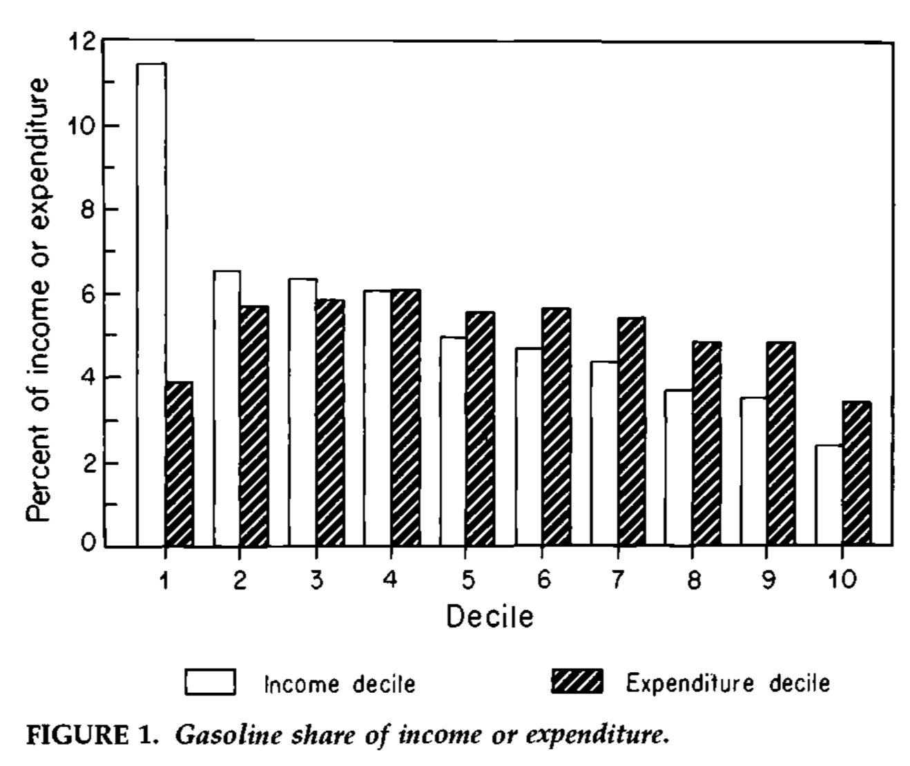
Who spends more on gasoline? One study by James Poterba (1991) suggests that the gasoline budget share is decreasing if we divide by income but not if we divide by all spending. The reason has to do with variation in how one defines disposable income (if for example one consumes out of savings).
To quantify income effects, we can use an income elasticity, provided variation in income is exogeneous, defined as
How do we find the elasticity from Marshallian demand? If we take the example above with \(X^* = \frac{I}{3p_X}\), then we apply the formula to get
\[\eta_{X,I} = \frac{1}{3 p_X}\frac{I}{\frac{I}{3p_X}} = 1\]
Marshallian demands from a Cobb-Douglas utility function always have unit income elasticity. Why? Because the budget share is fixed, \(s_X = \frac{p_X X^*(p_X,p_Y,I)}{I} = \alpha\) if \(u(X,Y) = X^{\alpha} Y^{1-\alpha}\). If income increases by 10%, demand increases by 10% so that the budget share of X remains constant. Hence, the cobb-douglas utility function is very restrictive and may not fit the data very well.
In practice, it is hard to observe the income elasticity because variation in income is rarely exogenous. What sort of events could you exploit? Maybe compare the consumption of lottery winners to non-winners or their own consumption over time. Maybe use bequests? The COVID-19 pandemic?
Provided variation in income is exogeneous, we can use a simple trick to estimate an elasticity. If we assume the elasticity is constant, then consider the relationship
where \(i\) denotes an observation pair (from data over individuals or time) and \(\epsilon_{i}\) is a noise term. Then, we have that
but also that
Therefore \(\beta\) is equal to \(\eta_{X,I}\). Hence, an income elasticity can be estimated from the slope of a linear regression of log quantity (or spending) of a good on log income. This constant elasticity specification is often called the log-log specification of demand. An estimate of the elasticity is therefore
Todo
Play around with this example of Engle Curves from EconGraph.org
See also
When preferences vary across individuals and perhaps correlated with income, then a regression such as the one above will lead to a biased estimate of the income elasticity as it confounds variation in spending from income which comes from income itself and variation which comes from variation in preferences. The sign of the bias depends on the relationship between income and preferences.
Price Effects
How do the demands \(X^*\) et \(Y^*\) change if \(p_Y\) and \(I\) stay constant but \(p_X\) changes?
To quantify this effect, we may use a price elasticity of the form:
This elasticity is invariant to monetary units.
So how do we compute it from Marshallian demands? Follow the definition and substitute the demand function,
The price elasticity is 1 (in absolute value). Again, this is because of the constant budget share restriction. If the price of good X increases by 10%, demand needs to decrease by 10% so that the budget share stays constant. Hence, if this utility function is what drives demand for a good, an additional tax does not raise additional revenue as expenditures on the good do not change! This is very restrictive.
To infer the price elasticity, a challenge is to find an experiment where the price is varied exogenously while other factors are kept constant. Taxation is one of the key source of variation exploited. Other examples include using supply shocks which lead to a change in the price not driven by demand. The log-log regression framework above can be used to estimate the price elasticity.
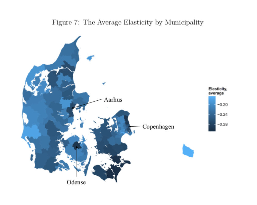
In Denmark, one study shows that the price elasticity varies a lot across the country and in particular reacts to the distance people need to travel to work and transportation alternatives they face.
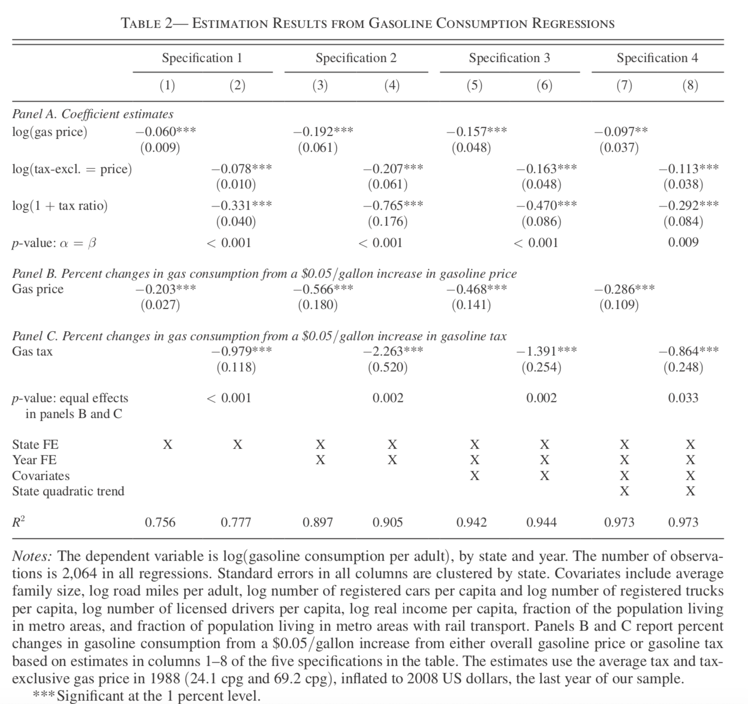
In the U.S., another analysis shows that a distinction should be made between a price change and a tax change. The effect of a tax appears to be more visible and people react more to it.
An increase in the price (or tax) has a direct effect of lowering utility. One may want to compensate households for this. To compute the compensation, we have to decompose the effect of a price increase into two forces.
There are two forces:
Public transportation is more affordable than the car (gasoline): consumers will want to substitute towards public transportation. This is a substitution effect which comes from the relative price signal.
\[\frac{u'_X(X,Y)}{u'_Y(X,Y)} = \frac{p_X}{p_Y}\]At current consumption, one needs more income to buy this basket at the new prices. Hence, the consumer needs to reduce his consumption: income effect.
Compensation will be a function of income and substitution effects. Hence, our objective: is to identify these effects and see how they lead to the total price effect.
Substitution and Income Effects in Action
Watch this podcast with Justin Caron, Associate Professor of Economics at HEC Montreal, on the effects of Carbon Taxes. Spot substitution and income effects in the discussion.
Compensated Demand
Compensated demand allows to separate substitution and income effects and understand better price effects.
Context
Reference price \((p_X,p_Y)\), reference income \(I\)
New prices \((\hat p_X,p_Y)\), income does not change.
Reference Demand, \(X(p_X,p_Y,I)\), indirect utility level at reference price and income \(v(p_X,p_Y,I)\)
New Demand, \(X(\hat p_X, p_Y, I)\), new indirect utility level \(v(\hat p_X,p_Y,I)\).
Compensated Income: income \(I^{cmp}\) such that we maintain utility at reference levels despite facing new prices.
\[v(p_X,p_Y, I) = v(\hat p_X, p_Y, I^{cmp})\]
Compensated demand (or hicksian) is given by the marshallian demand where we replace income by compensated income \(X^{cmp}= X(\hat p_X, p_Y, I^{cmp})\).
Todo
Exercise A: Compute compensated income and demand for \(X\) if \(u(X,Y) = XY\) and \(p_X X+p_Y Y \le I\) for a price change \(\hat p_X > p_X\).
Todo
Play around with this example of compensating variation from EconGraph.org.
Todo
Play around with this example of Marshallian and Hicksian Demand from EconGraph.org.
See also
There exist a dual theory of consumer choice which alternatively derives the compensated demand from minimizing expenditures subject to maintaining utility above a certain level. We do not do this here.
Important
Compensated income for a price increase is always higher than reference income. The difference is the compensation required. If the price increase results from a tax, this new compensation is required not to make consumers worse off. Yet, even if the compensation occurs, it still has the potential of changing behavior: a price change results in a potential substitution effect which does not go away if compensation occurs.
Important
Law of Compensated Demand If \(\hat p_X > p_X\), then \(X^{cmp}(p_X,p_Y,I)<X(p_X,p_Y,I)\). Compensated demand for \(X\) is decreasing in the price \(p_X\).
We can compute the compensation required (and compensated income) for more general problems. We start by specifying demand and indirect utility:
def x_d(p_x,p_y,I,alpha):
   return alpha*I/p_x
def y_d(p_x,p_y,I,alpha):
   return (1-alpha)*I/p_y
def v(p_x,p_y,I,alpha):
   xstar = x_d(p_x,p_y,I,alpha)
   ystar = y_d(p_x,p_y,I,alpha)
   return u(xstar,ystar,alpha)
We then exploit the following equation that defines the compensation:
We are looking for \(I^{cmp}\) which makes the difference between the left and right hand side as small as possible. We can write that function (the main argument here is the compensation \(\Delta I^{cmp} = I^{cmp} - I\)):
def slack(cmp,p_x,dp_x,p_y,I,alpha):
   return v(p_x,p_y,I,alpha) - v(p_x+dp_x,p_y,I+cmp,alpha)
If we evaluate at zero, we will return a value which is positive (the consumer does not like an increase in the price if dp_x>0), and if cmp is too large, we will have something negative (we are giving too much compensation). The objective is to find cmp such that the function slack() is zero. The bisect algorithm allows us to do that,
from scipy.optimize import bisect

cmp = bisect(slack,0,I,args=(p_x,dp_x,p_y,I,alpha))
The function returns the necessary compensation which is required for a change in the price dp_x. The notebook below gives a more involved example of this.
We can now define substitution and income effects, now that we are able to identify compensated income and demand.
Substitution Effect
Change in demand caused by a relative price change, keeping utility constant.
Substitution Effect \(=\) Compensated Demand - Reference Demand
\[\Delta X^{{cmp}} = X(\hat p_X,p_Y,I^{cmp}) - X(p_X,p_Y,I)\]
Income Effect
Change in demand caused by a change in purchasing power, keeping prices constant.
Income Effect \(=\) New demand - compensated demand
We can approximate the compensated income for a small change in price:
To keep notation light, denote
Then define \(I^{cmp}= I + \Delta I^{cmp}\), \(X^{cmp}= X^* + \Delta X^{cmp}\) and \(Y^{cmp}= Y^* + \Delta Y^{cmp}\).
Therefore,
Why does \(p_X\Delta X^{{cmp}} + p_Y \Delta Y^{{cmp}} = 0\)?
\((X^*,Y^*)\) and \((X^{cmp},Y^{cmp})\) are on the same indifference curve and close to each other for a small price change, which implies,
\[\frac{\Delta Y^{cmp}}{\Delta X^{cmp}} = MRS_{X}\]
\((X^*,Y^*)\) is optimal at prices \(p_X, p_Y\), which implies \(MRS_{X} = -\frac{p_X}{p_Y}\). Therefore, \(p_X \Delta X^{cmp}+ p_Y \Delta Y^{cmp}= 0\).
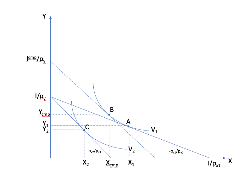
In the \((X,Y)\) space, consider a price increase for good \(X\). The index 1 refers to the reference situation and index 2 to the situation with the new prices. The consumer is initially at point A (reference). With the price change, the budget constraint has a steeper slope. After the price change, the consumer is at price C. To decompose this price change, we compensate the consumer at the new prices. He chooses point B, with the same utility as in the reference situation. The passage from A to B is the substitution effect. The passage from B to C is the income effect. The sum of the two yield the total effect of the price change.
Todo
Exercise B: See if this is a good approximation for \(U(X,Y) = XY\) with reference price and income \((p_X,p_Y,I) = (1,1,100)\) and \(\Delta p_X = 1\). Find the substitution and income effects.
Todo
Play around with this Example of Decomposition of a Price Change (lower price) from EconGraph.org.
Slutsky Equation
The Slutsky equation allows to look the total price effect, the substitution effect and the income effect. The first and the last is observable given sufficient exogenous variation. The second one is necessary to compute the compensation required.
To keep notation simple, consider
We get
Since
then,
In terms of elasticities, we multiply both sides by \(\frac{p_X}{\Delta p_X X^*}\) and we multiply the last term by \(I/I\). We get,
Finally, we note that \(\frac{\partial X}{\partial I} = \eta_{X,I}\frac{X^*}{I}\). Replacing and denoting the budget share of \(X\) as \(s_X = \frac{p_X X^*}{I}\), the Slutsky equation becomes:
Todo
Exercise C: For Cobb-Douglas preferences \(U(X,Y) = X^\alpha Y^{1-\alpha}\), compute compensated price elasticity using the Slutsky equation.
Cross-price Effects
The nature of goods, complements or substitutes is determined by how they compensated demands (not marshallian) react to cross-price changes. Compensated demands are necessary to define those precisely. Goods \(X\) and \(Y\) are:
Substitutes: if the cross-price effect is positive: \(\frac{\partial X^{cmp}}{\partial p_Y} >0\)
Complements: If the cross-price effect is negative: \(\frac{\partial X^{cmp}}{\partial p_Y} <0\)
Todo
What is your prior about the cross-price elasticity of public transportation? How would it factor into your analysis of a policy that taxes gasoline to reduce carbon emissions?
Properties of Demand Functions
Demand functions have certain properties which follow directly from the axioms controlling preferences and utility maximization:
Homogeneity of degree zero (no monetary illusion)
\[X(\lambda p_X,\lambda p_Y,\lambda I) = X(p_X,p_Y,I)\]Symmetry:
\[\frac{\partial X^{cmp}}{\partial p_Y} =\frac{\partial Y^{cmp}}{\partial p_X}\]Additivity:
\[p_X \frac{\partial X(p_X,p_Y,I)}{\partial I} + p_Y \frac{\partial Y(p_X,p_Y,I)}{\partial I} = 1\]Negativity (Law of compensated demand):
\[\frac{\partial X^{cmp}}{\partial p_X}<0,\frac{\partial Y^{cmp}}{\partial p_Y}<0\]
Price indices of Cost-of-Living
To measure how the cost-of-living changes, we use consumer price indices (CPI). One such index is the Laspeyres index:
Note that \(X\) and \(Y\), bought in the reference situation, are also used after the price change. This CPI keeps quantities fixed, at least in the short term. The policy question is that many government benefits are indexed to the CPI and it is not clear whether the CPI really reflects changes in purchasing power. The objective of this indexation is to maintain power purchasing power of these benefits constant but it does not account for the fact that consumers substitute away from goods whose price increases more, in relative terms. Another issue is that monetary policy is also based on inflation which is measured using the CPI.
For an increase in the price of \(X\), the effect on purchasing power can be measured with:
\[\pi_I = \frac{I^{cmp}}{I}\]
This will depend on preferences. It is possible that this Hicksian price index yields a different answer than the Laysperes price index. In particular, if the income share of a good decrease when its price increase, the Hicksian index often yields a lower increase in the cost-of-living than what the Laysperres index would suggest. We call this bias the substitution bias in price indices.
Before the pandemia hit and a lockdown was imposed, gasoline consumption went down. The price of gas also decreased (for may reason). Does a Laysperes index give a good indication of the change in purchasing power during this period? This article does the computation for the U.S. and shows that inflation is underestimated.
Pricing and Demand Analysis
Why would a firm study properties of the demand it faces? Because it can potentially increase sales if it has market power, an ability to affect or manipulate the price on the market. Firms can also price discriminate: segment the market or offer bundles at different prices. They can exploit complementarities between goods to offer bundles. All of this requires good knowledge of demand.
See also
The Orbitz scandal occured because it was revealed that Orbitz, an online platform for hotels, was presenting higher prices to Mac users than to PC users. This is based on the fact that Mac users where often willing to pay more for accomodation. They were less price sensitive. This shows how firms can use demand information to price their products differentially. In the lectures on Imperfect competition, we will show how this information can be used. It is also a communications nightware when it becomes public…
Econometric analysis can be used along with some theory, to extract information from firm and market data. In the retail industry, firms purchase for example scanner data to learn about consumers and their sensitivity to prices.
Python example
See this notebook which uses the CES utility function to study price and income effects.
![]()