Time¶

Preferences¶

Generally, everyone prefers to get benefits as fast as possible and incur cost as late as possible:

A coffee now or in an hour?
Go to the Gym today or tomorrow?
Save now or next year?

Empirical evidence suggest that the origin of preferences can be traced to childhood. But preferences may change over time.

Discounted Utility¶

In his book The Theory of Interest in 1930, Irving Fisher presents a simple theory which is the foundation to modern finance and macro. Preferences are represented using discounted utility.

If $u(C_t)$ denotes utility of consuming in period $t$, discounted utility for a consumption plan $\textbf{C} = (C_1,...,C_T)$ is :

\[DU(\mathbf{C}) = \sum_{t=1}^T \delta^{t-1} u(C_t)\]

$\delta$ $\in [0,1]$ is the discount factor (higher value indicates patience). The relationship between the discount rate $\rho$ and the discount factor is given by:

\[\delta = \frac{1}{1+\rho}\]

Marginal Rate of Substitution (MRS)¶

If $T=2$, then

\[DU(C_1,C_2) = u(C_1) + \delta u(C_2)\]

Total differentiating to obtain the MRS yields:

\[\frac{\partial C_2}{\partial C_1}\rvert_{dDU=0} = -\frac{u'(C_1)}{\delta u'(C_2)}\]

Important

Intertemporal preferences are captured by the discount factor ($\delta$) and the shape of $u$.

Todo

Exercise A: Find the MRS for $u(C_t) = \log C_t$

How can we estimate the discount rate (factor)? We can use MPL (see course on risk).

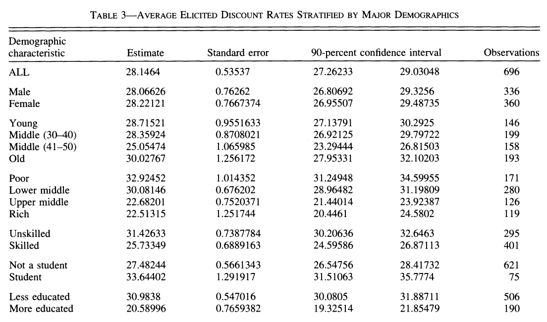
A Danish study estimates discount rates using MPL (Harrison, Lau and Williams, 2002)

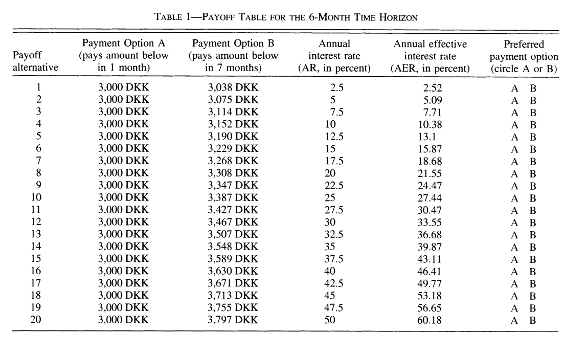
Results show great dispersion and high discount rates, much higher than interest rates.

Intertemporal Budget Constraint¶

Interest and Financial Markets

Financial institutions offer $r_S$ for each dollar deposited (savings). We are asked $r_D$ for each dollar borrowed.

Assume for the moment that $r_D = r_S = r$.

Resources

Resources originate from:

Initial wealth: $W_0$.
Income during both periods $Y_1$, $Y_2$.

The present value (PV) of these resources :

\[PV_W = W_0 + Y_1 + \frac{Y_2}{1+r}\]

Constraint

Present value of consumption is given by:

\[PV_C = C_1 + \frac{C_2}{1+r}\]

Therefore, the budget constraint is $PV_C \leq PV_W$:

\[C_1 + \frac{C_2}{1+r} \leq W_0 + Y_1 + \frac{Y_2}{1+r}\]

Borrowing and Saving

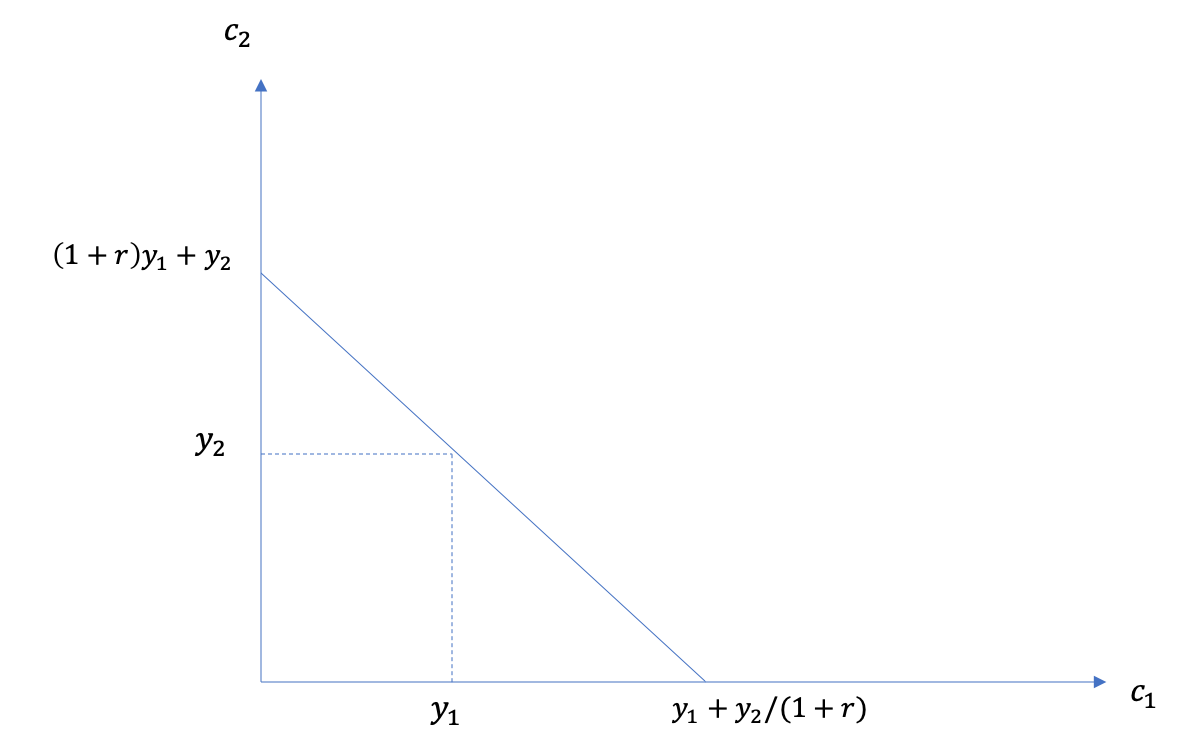
We can write the constraint as

\[(1+r)(W_0 + Y_1 - C_1) \ge C_2 - Y_2\]

Important

If one saves in the first period, one can also consume more than income in the second period. An individual who borrows in the first period has to consume less than his income in the second period.

Visually, we have

Todo

Play around with the budget constraint at EconGraph.org.

Example: We can incorporate a pension plan into our budget constraint. A defined benefit pension plan forces the individual to save in the first period (contribute) against a fixed pension benefit in the second period.

Income in the second period is $Y_2 = \phi Y_1$ with a replacement rate $\phi \in [0,1]$.
Income in th first period is reduced by the contribution to the pension plan $\tau Y_1$.

The budget constraint is:

\[C_1 + \frac{C_2}{1+r} \leq W_0 + (1-\tau)Y_1 + \frac{\phi Y_1}{1+r}\]

Actuaries pick the contribution rate $\tau$ such that:

\[\tau Y_1 = \frac{\phi Y_1}{1+r_P} \to \tau = \frac{\phi}{1+r_P}\]

where $r_P$ is the implicit return of the pension fund. If $r_P = r$, the budget constraint is identical! The consumption plan does not change and so private savings is reduced one to one with the contribution made (crowdout effect). Lots of research is devoted to understanding the interplay between pensions and savings.

Spread between returns and borrowing costs

Todo

Exercise B: What does the budget constraint look like if $r_S<r_D$?

Todo

Exercise C: How to represent a situation where the agent cannot borrow?

Optimal Choice¶

Maximization

The problem is (fix $W_0=0$ to simplify):

\[\max_{C_1,C_2} \{ u(C_1) + \delta u(C_2) : C_1+C_2/(1+r) \leq Y_1 + Y_2/(1+r)\}\]

Two approaches:

Direct approach (substitution of constraints)
Lagrangian

Optimality conditions

The Lagrangian has three FOC:

\[\begin{split}\begin{aligned} u'(C_1) - \lambda = 0 \\ \delta u'(C_2) - \lambda /(1+r) = 0 \\ C_1+C_2/(1+r) - Y_1 - Y_2/(1+r) = 0 \end{aligned}\end{split}\]

With (1) and (2) we get :

\[\frac{u'(C_1)}{\delta u'(C_2)} = 1+r\]

Important

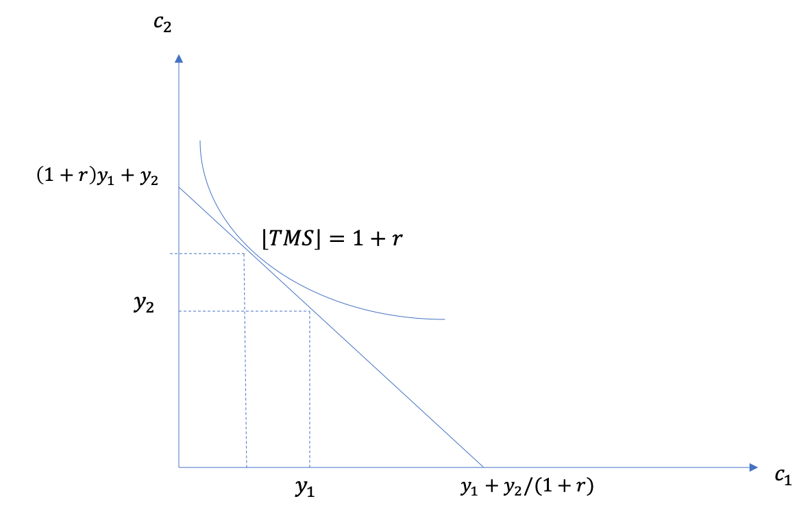
The consumer picks his consumption level such that the value of increasing current consumption (MRS) is equal to the opportunity cost of doing it in terms of second period consumption.

Todo

Play around with the optimality condition at EconGraph.org.

We can rearrange, fixing $R=1+r$, to obtain the Euler equation:

\[u'(C_1) = R\delta u'(C_2)\]

Visually,

This theory is the basis for the life-cycle model (the Life-Cycle Hypothesis), proposed by Franco Modigliani, which allows to understand decisions over age. The agent prefers to smooth the marginal utility of consumption over the life-cycle. If he has high income while young and lower income when older, he has low marginal utility of consumption when young and high marginal utility when old if he simply consumes his income. Optimally, he will want to consume less when young (save) to increase is marginal utility of consumption and consume more when old (to lower his marginal utility of consumption). This is the basis of why consumers demand pensions and private savings.

Todo

Exercise D: Find the optimal choice $C_1$ and $C_2$ if $u(C)=\frac{C^{1-\sigma}}{1-\sigma}$ and the consumer faces the classic budget constraint above.

Example: Are Canadians saving enough for retirement?

A question often making headlines.

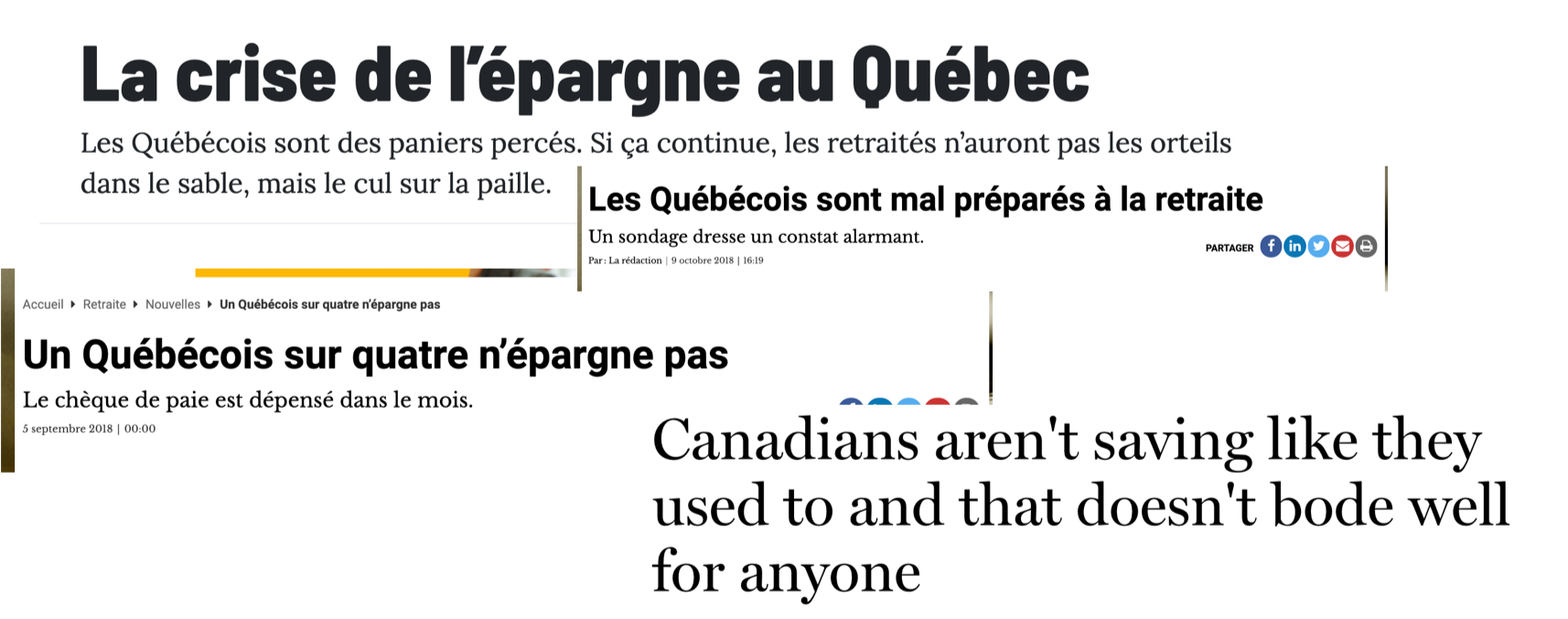
Le Conseiller, Globe and Mail, L’Actualité¶

This is a difficult question. One can simulate outcomes using very sophisticated models but how do we determine what is enough? Is saving too much also a problem?

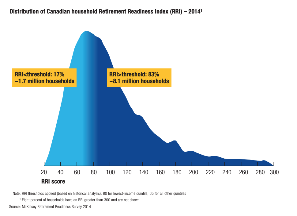
McKinsey (2015)¶

For more recent calculations, see this report of the Retirement and Savings Institute at HEC.

Optimal Savings

What does theory tell us about optimal savings?

Todo

Exercise E: Find the solution for optimal savings at the beginning of period 2 if $u(C)=\frac{C^{1-\sigma}}{1-\sigma}$ and the budget constraint is given by :

\[C_1 + \frac{C_2}{1+r} \leq (1-\tau)Y_1 + \frac{\phi Y_1}{1+r}\]

More sophisticated computations can be done to compute how much people should save and compare it to how much they have actually saved:

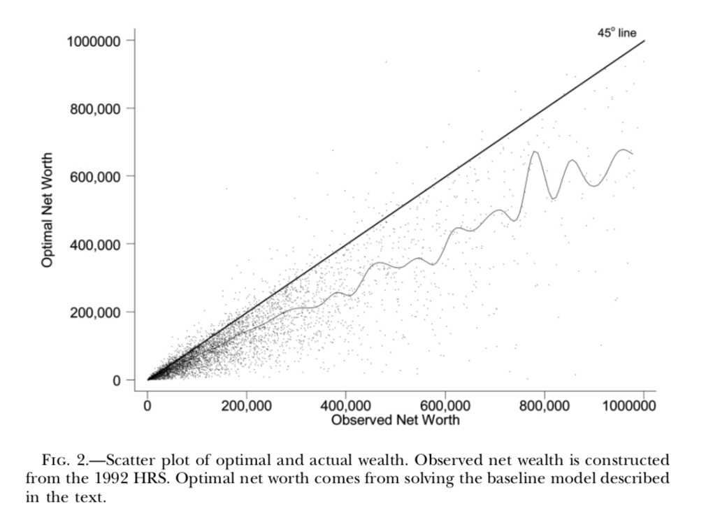
Scholz et al. (2007, Journal of Political Economy)¶

Conclusions are sometimes surprising compared to what we hear in the media. A vast majority appears to save enough. Some even save too much.

Microeconomics in Action: Saving for Retirement

Watch this podcast with Bernard Morency, adjunct Professor at HEC Montreal and world-renowned expert on retirement.

Present bias¶

As we have seen, individuals can be very impatient. But their preferences may still fit discounted utility theory. There is no contradiction. But there exist violations of discounted utility which have to do with the way people discount the very short term and the medium and long-term. If the discount function is not exponential, but rather hyperbolic for example, then individuals make inconsistent plans which they will not follow upon.

Example: Picking a movie

You have to pick one movie to watch today and one you will watch next week:

Assume, Mommy has an immediate benefit of 4 and also a future benefit of 4 but that Les Boys has an immediate benefit of 7 (but no future benefit).

Todo

Exercise F: What is your discounted utility if you pick a movie today and $\delta=1$. What happens if we delay movie watching to next week but you have to pick today?

Empirical evidence suggests that in such choice situations, lots of people will pick Les Boys if they watch tonight. If they pick for next week today, they will pick Mommy. Discounted utility does not allow for such choice reversals, what is often called dynamic inconsistency.

Present-Bias and Quasi-Hyperbolic Preferences

Laibson (1997, QJE) proposes a simple modification to discounted utility, but with major implications. He produces to use a quasi-hyperbolic discount faction that discounts more heaviliy the immediate short term than the long-term:

\[QH(\mathbf{c}) = u(C_1) + \beta \sum_{t=2}^T \delta^{t-1} u(C_t)\]

The parameter $\beta$ acts as a measure of present bias (the lower it is, the larger the bias) while $\delta$ controls impatience in the long-term (similar to discounted utility discount factors). These preferences depend on the horizon.

Todo

Exercise G: What is the MRS between $C_1$ and $C_2$? And $C_2$ vs. $C_3$? Compare with discounted utility.

Using the two movie example, assume now $\beta=0.5$.

Todo

Exercice H: Repeat Exercise F. Which film do you now pick for this week and next week if you have quasi-hyperbolic preferences? What do you do when next week comes?

Example: Who buys Annual Gym memberships?

Della Vigna et Malmendier (2006) study the choice between taking an annual membership to a Gym vs. purchasing individual passes valid for one visit to the Gym. An daily pass costs 10$. But given how rarely some people go to the gym, those who purchase an annual membership often end up paying much more per visit. Why do they buy the membership? Don’t they know that they may suffer from present-bias?

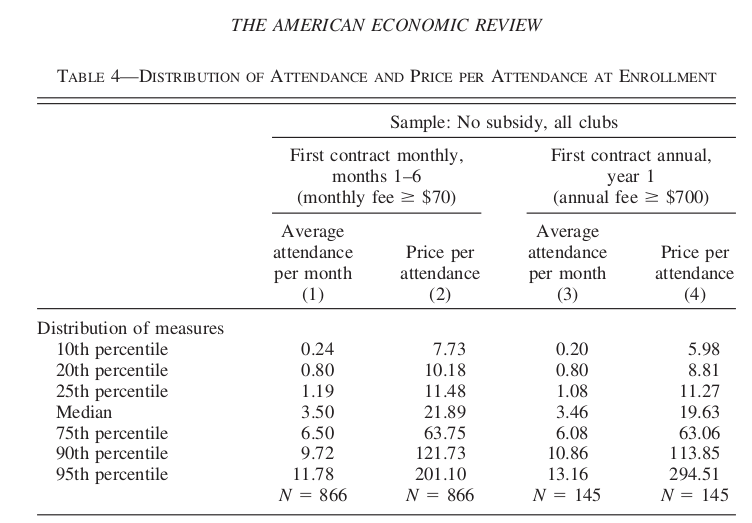
There is evidence that many underestimate their degree of present bias. Some models have been constructed to capture this degree of naiveté.

Example: How do we help people to save?

Saving is, in some respects, similar to going to the Gym: costly in the short-term (sacrifice consumption), benefits in the long-term (future consumption).
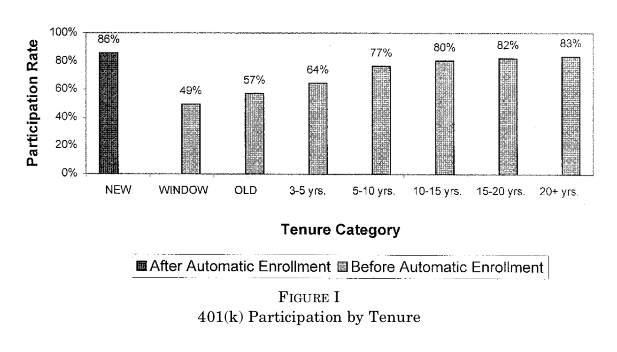
To help people with these biases, nudges can be used. Turns out that making people do something by default increases retention into a particular behavior.
Shea et Madrian (2001, QJE) is a famous example. Moving from opt-in to opt-out increases participation in a pension plan.

Shea et Madrian (2001, QJE)¶

Commitment

People who have present-bias may have a demand for devices that help them keep their future selves in check… David Laibson and may others, study mechanisms of this sort, applied to savings and health for example.

Intertemporal Choice Python¶

Here is Python example.